This function summarizes code counts and their proportional representation across media titles (e.g., interviews, focus groups, or other qualitative data sources). It can optionally produce a formatted table and/or a ggplot visualization showing saturation by code frequency or proportion.
Arguments
- code_counts
A tibble or data frame containing columns:
code: the code labelcount: total number of excerpts coded with that coden_media_titles: number of distinct media titles (e.g., transcripts) in which the code appears. This object is typically generated bycreate_code_summary().
- total_media_titles
Optional numeric value indicating the total number of media titles. If
NULL(default), the function uses the maximum value ofn_media_titles.- table_min_count
Minimum count threshold for including a code in the output table. Defaults to 1.
- table_min_prop
Minimum proportion threshold (relative to total media titles) for including a code in the output table. Defaults to
NULL(no proportion filter).- output_type
Character string indicating the output format for the table: either
"tibble"(default) or"kable".- plot
Logical; if
TRUE, produces a ggplot visualization. Defaults toFALSE.- plot_min_count
Minimum count threshold for codes to include in the plot. Defaults to
table_min_countifNULL.- plot_min_prop
Minimum proportion threshold for codes to include in the plot. Defaults to
table_min_propifNULL.- plot_metric
Character string indicating what to plot:
"prop"for proportions,"count"for counts, or"both"for dual-axis plot. Defaults to"prop".- fill_color
Character string specifying the fill color for bars in the plot. Defaults to
"steelblue".
Value
If
plot = FALSE: returns a tibble (or kable table) summarizing code frequencies and proportions.If
plot = TRUE: returns a list with two elements:table: the filtered tibbleplot: a ggplot2 object.
Examples
# Example dataset
code_counts <- tibble::tibble(
code = c("Belonging", "Resilience", "Stress", "Hope"),
count = c(15, 10, 8, 5),
n_media_titles = c(8, 6, 5, 3)
)
# Basic usage (returns a tibble)
set_saturation(code_counts)
#> # A tibble: 4 × 3
#> code count prop_media_titles
#> <chr> <dbl> <dbl>
#> 1 Belonging 15 1
#> 2 Resilience 10 0.75
#> 3 Stress 8 0.62
#> 4 Hope 5 0.38
# Apply count and proportion filters, return a kable table
set_saturation(
code_counts,
total_media_titles = 10,
table_min_count = 5,
table_min_prop = 0.3,
output_type = "kable"
)
#>
#>
#> Table: Code Counts with Transcript Proportions (table_min_count = 5 , table_min_prop = 0.3 )
#>
#> |code | count| prop_media_titles|
#> |:----------|-----:|-----------------:|
#> |Belonging | 15| 0.8|
#> |Resilience | 10| 0.6|
#> |Stress | 8| 0.5|
#> |Hope | 5| 0.3|
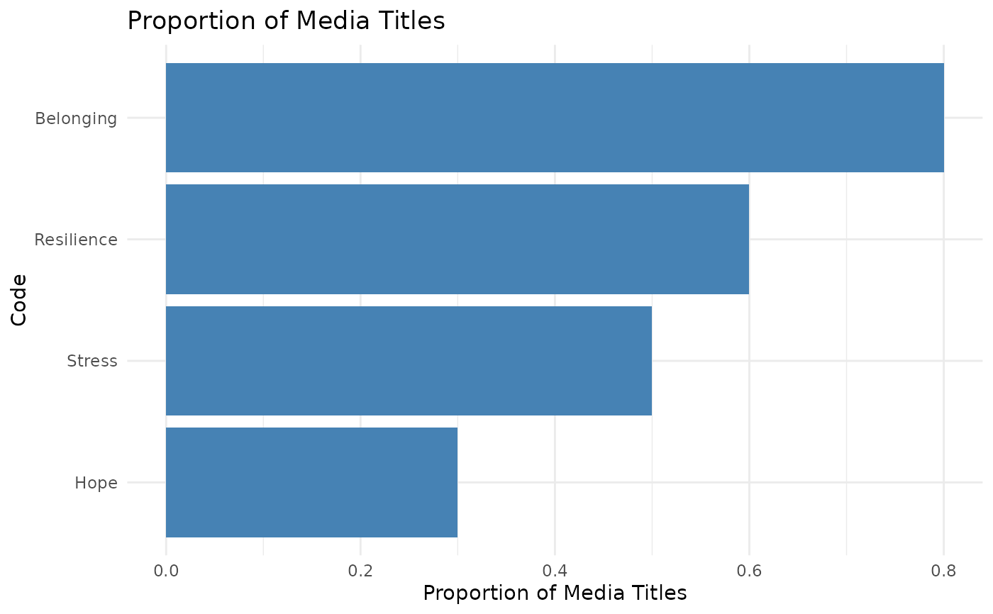
# Generate a plot of proportions
res <- set_saturation(
code_counts,
total_media_titles = 10,
plot = TRUE,
plot_metric = "prop"
)
res$plot
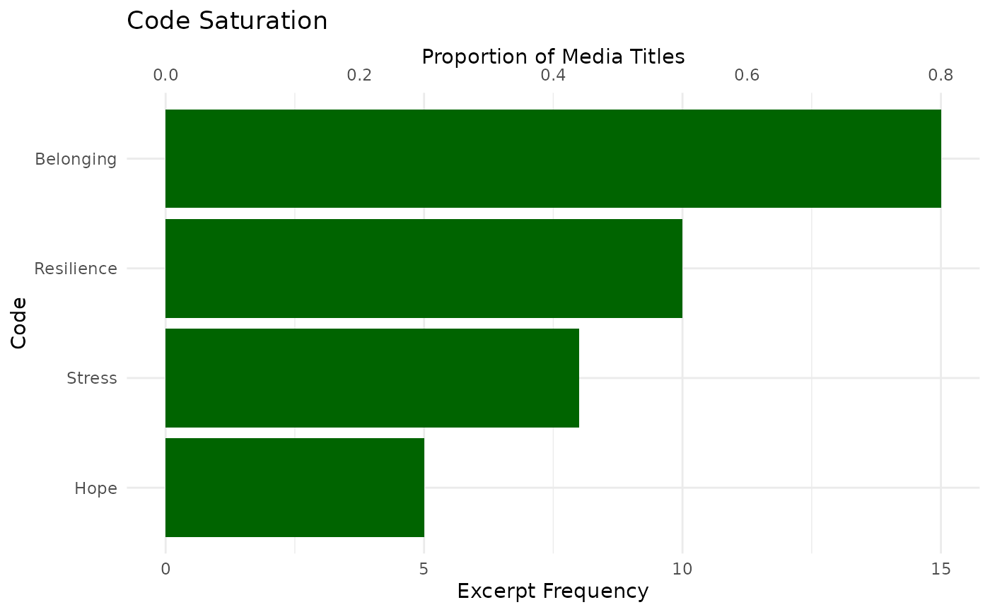
 # Plot both count and proportion using dual y-axes
res <- set_saturation(
code_counts,
total_media_titles = 10,
plot = TRUE,
plot_metric = "both",
fill_color = "darkgreen"
)
res$plot
# Plot both count and proportion using dual y-axes
res <- set_saturation(
code_counts,
total_media_titles = 10,
plot = TRUE,
plot_metric = "both",
fill_color = "darkgreen"
)
res$plot